An Approximate Exponentiated Weibull Joint Envelope-Phase Distribution

Talk on free space optical channels at the IEEE APS Meeting 2016

Transcript

1. Introduction Joint Envelope-Phase Probability Density Function Conclusions An Approximate Exponentiated Weibull Joint Envelope-Phase Distribution José V. M. Cardoso, Wamberto J. L. Queiroz, and Marcelo S. Alencar Institute for Advanced Studies in Communications – Iecom Department of Electrical Engineering Federal University of Campina Grande – UFCG IEEE AP-S/URSI 2016 Fajardo, Puerto Rico 1 / 15 An Approximate Exponentiated Weibull Joint Envelope-Phase Distribution IEEE AP-S/URSI 2016
2. Introduction Joint Envelope-Phase Probability Density Function Conclusions Outline 1 Introduction Atmospheric Turbulence Channel Statistics 2 Joint Envelope-Phase Probability Density Function 3 Conclusions 2 / 15 An Approximate Exponentiated Weibull Joint Envelope-Phase Distribution IEEE AP-S/URSI 2016
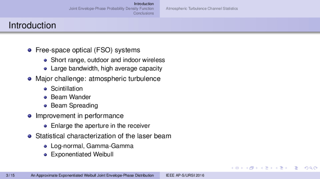
3. Introduction Joint Envelope-Phase Probability Density Function Conclusions Atmospheric Turbulence Channel Statistics Introduction Free-space optical (FSO) systems Short range, outdoor and indoor wireless Large bandwidth, high average capacity Major challenge: atmospheric turbulence Scintillation Beam Wander Beam Spreading Improvement in performance Enlarge the aperture in the receiver Statistical characterization of the laser beam Log-normal, Gamma-Gamma Exponentiated Weibull 3 / 15 An Approximate Exponentiated Weibull Joint Envelope-Phase Distribution IEEE AP-S/URSI 2016
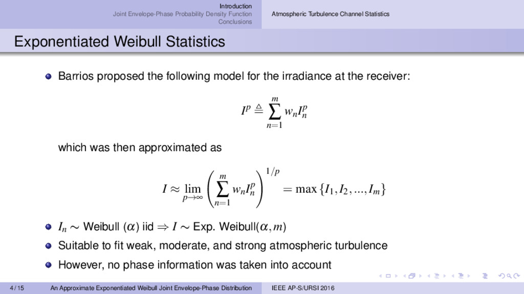
4. Introduction Joint Envelope-Phase Probability Density Function Conclusions Atmospheric Turbulence Channel Statistics Exponentiated Weibull Statistics Barrios proposed the following model for the irradiance at the receiver: Ip m ∑ n=1 wn Ip n which was then approximated as I ≈ lim p→∞ m ∑ n=1 wn Ip n 1/p = max{I1,I2,...,Im} In ∼ Weibull (α) iid ⇒ I ∼ Exp. Weibull(α,m) Suitable to fit weak, moderate, and strong atmospheric turbulence However, no phase information was taken into account 4 / 15 An Approximate Exponentiated Weibull Joint Envelope-Phase Distribution IEEE AP-S/URSI 2016
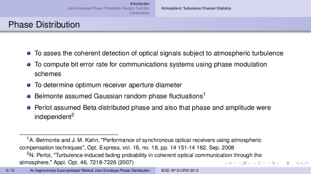
5. Introduction Joint Envelope-Phase Probability Density Function Conclusions Atmospheric Turbulence Channel Statistics Phase Distribution To asses the coherent detection of optical signals subject to atmospheric turbulence To compute bit error rate for communications systems using phase modulation schemes To determine optimum receiver aperture diameter Belmonte assumed Gaussian random phase fluctuations1 Perlot assumed Beta distributed phase and also that phase and amplitude were independent2 1A. Belmonte and J. M. Kahn, "Performance of synchronous optical receivers using atmospheric compensation techniques", Opt. Express, vol. 16, no. 18, pp. 14 151-14 162, Sep. 2008 2N. Perlot, "Turbulence-induced fading probability in coherent optical communication through the atmosphere," Appl. Opt. 46, 7218-7226 (2007) 5 / 15 An Approximate Exponentiated Weibull Joint Envelope-Phase Distribution IEEE AP-S/URSI 2016
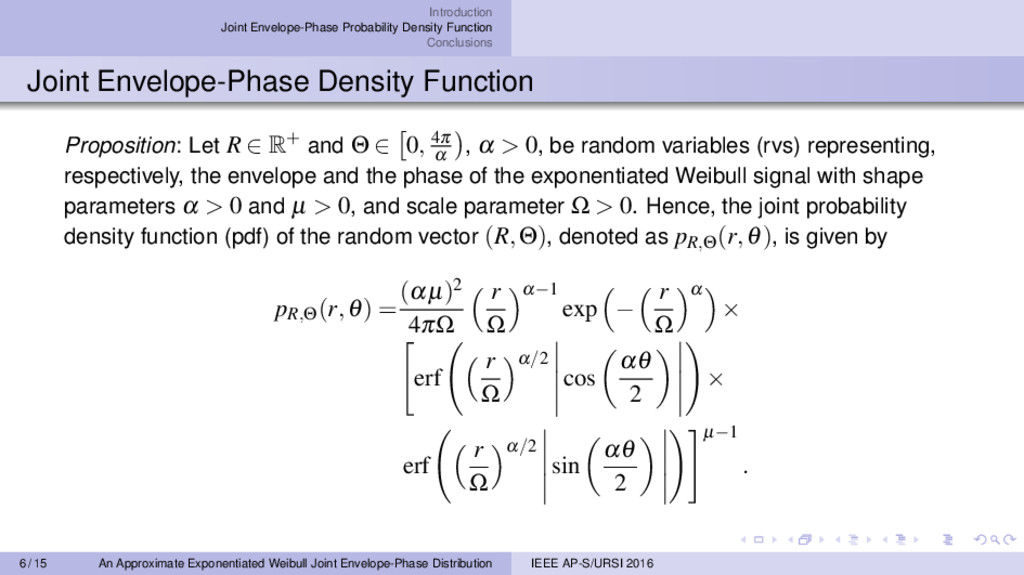
6. Introduction Joint Envelope-Phase Probability Density Function Conclusions Joint Envelope-Phase Density Function Proposition: Let R ∈ R+ and Θ ∈ 0, 4π α , α > 0, be random variables (rvs) representing, respectively, the envelope and the phase of the exponentiated Weibull signal with shape parameters α > 0 and µ > 0, and scale parameter Ω > 0. Hence, the joint probability density function (pdf) of the random vector (R,Θ), denoted as pR,Θ(r,θ), is given by pR,Θ(r,θ) = (αµ)2 4πΩ r Ω α−1 exp − r Ω α × erf r Ω α/2 cos αθ 2 × erf r Ω α/2 sin αθ 2 µ−1 . 6 / 15 An Approximate Exponentiated Weibull Joint Envelope-Phase Distribution IEEE AP-S/URSI 2016
7. Introduction Joint Envelope-Phase Probability Density Function Conclusions Joint Envelope-Phase Density Function Proof: R ∈ R+, Θ ∈ 0, 4π α , α ∈ R+ Z = X +jY Rα/2 exp jαΘ 2 X = Rα/2 cos αΘ 2 ; Y = Rα/2 sin αΘ 2 X2 max 1≤i≤m X2 i and Y2 max 1≤i≤m Y2 i , m ∈ N, in which Xi and Yi are assumed to be independent Gaussian distributed rvs with zero mean and variance Ωα 2 , representing the scattered fields in the in-phase and quadrature components, respectively 7 / 15 An Approximate Exponentiated Weibull Joint Envelope-Phase Distribution IEEE AP-S/URSI 2016
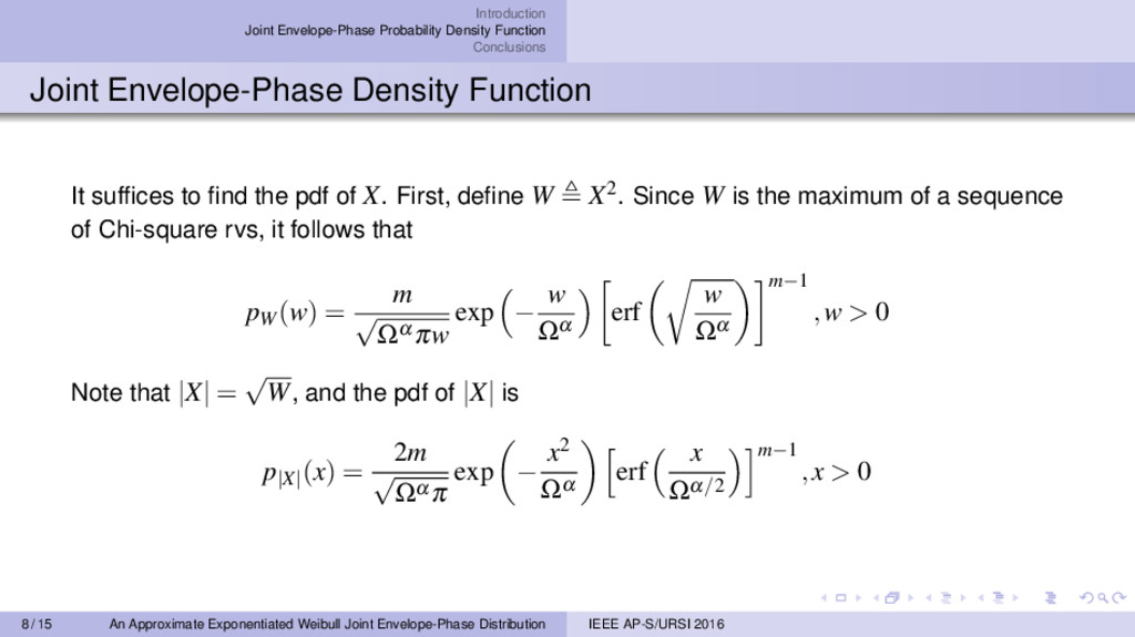
8. Introduction Joint Envelope-Phase Probability Density Function Conclusions Joint Envelope-Phase Density Function It suffices to find the pdf of X. First, define W X2 . Since W is the maximum of a sequence of Chi-square rvs, it follows that pW(w) = m √ Ωαπw exp − w Ωα erf w Ωα m−1 ,w > 0 Note that |X| = √ W, and the pdf of |X| is p |X| (x) = 2m √ Ωαπ exp − x2 Ωα erf x Ωα/2 m−1 ,x > 0 8 / 15 An Approximate Exponentiated Weibull Joint Envelope-Phase Distribution IEEE AP-S/URSI 2016
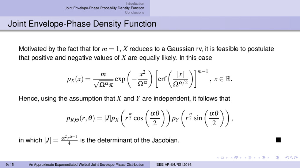
9. Introduction Joint Envelope-Phase Probability Density Function Conclusions Joint Envelope-Phase Density Function Motivated by the fact that for m = 1, X reduces to a Gaussian rv, it is feasible to postulate that positive and negative values of X are equally likely. In this case pX(x) = m √ Ωαπ exp − x2 Ωα erf |x| Ωα/2 m−1 , x ∈ R. Hence, using the assumption that X and Y are independent, it follows that pR,Θ(r,θ) = |J|pX rα 2 cos αθ 2 pY rα 2 sin αθ 2 , in which |J| = α 2rα−1 4 is the determinant of the Jacobian. 9 / 15 An Approximate Exponentiated Weibull Joint Envelope-Phase Distribution IEEE AP-S/URSI 2016
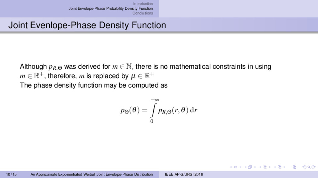
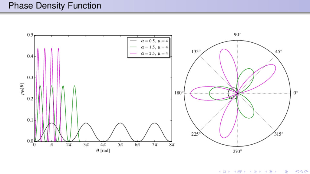
10. Introduction Joint Envelope-Phase Probability Density Function Conclusions Joint Evenlope-Phase Density Function Although pR,Θ was derived for m ∈ N, there is no mathematical constraints in using m ∈ R+, therefore, m is replaced by µ ∈ R+ The phase density function may be computed as p Θ(θ) = +∞ 0 pR,Θ(r,θ) dr 10 / 15 An Approximate Exponentiated Weibull Joint Envelope-Phase Distribution IEEE AP-S/URSI 2016
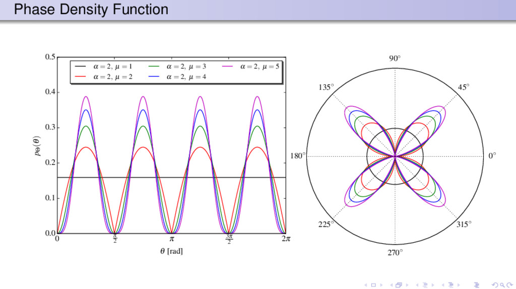
11. Introduction Joint Envelope-Phase Probability Density Function Conclusions Remarks As expected, in case µ = 1, pR,Θ reduces to the joint Weibull distribution For µ = 1 and α = 2, pR,Θ specializes to the joint Rayleigh distribution Apart from the case in which µ = 1, the envelope and the phase are not independent rvs Futhermore, the phase Θ is uniform if and only if µ = 1 11 / 15 An Approximate Exponentiated Weibull Joint Envelope-Phase Distribution IEEE AP-S/URSI 2016
12. Phase Density Function 0 π 2 π 3π 2 2π θ [rad] 0.0 0.1 0.2 0.3 0.4 0.5 p Θ(θ) α = 2, µ = 1 α = 2, µ = 2 α = 2, µ = 3 α = 2, µ = 4 α = 2, µ = 5 0◦ 45◦ 90◦ 135◦ 180◦ 225◦ 270◦ 315◦
13. Phase Density Function 0 π 2π 3π 4π 5π 6π 7π 8π θ [rad] 0.0 0.1 0.2 0.3 0.4 0.5 p Θ(θ) α = 0.5, µ = 4 α = 1.5, µ = 4 α = 2.5, µ = 4 0◦ 45◦ 90◦ 135◦ 180◦ 225◦ 270◦ 315◦
14. Introduction Joint Envelope-Phase Probability Density Function Conclusions Conclusions and Future Works A novel, approximate, and closed-form expression for the exponentiated Weibull joint envelope-phase distribution has been derived The exponentiated Weibull model fading finds applications in free-space optical communications channels subject to a variety of atmospheric turbulence conditions The proposed joint distribution may be applied to determine the performance, reliability, and high order statistics of such communications channels in many scenarios Further investigations may be conducted to derive an analytical expression for the marginal phase density function and to validate it with experimental data 14 / 15 An Approximate Exponentiated Weibull Joint Envelope-Phase Distribution IEEE AP-S/URSI 2016
15. Acknowledgments Contact: jvmirca@gmail.com